There are a lot abandoned structures in the desert, some hundreds of years old, which are always fun to visit. Trying to find them, however, is a very tedious process of scanning Google satellite imagery.
This project was an attempt to speed up the process with a custom model trained for oriented bounding box labeling of public LiDAR data.
// Why Public Data
While there are many services offering high-resolution satellite imagery on demand, these services are usually oriented towards property developers and companies looking to monitor their overseas operations and the pricing, as much as $10,000, reflects that.
Additionally, there are limits to what can be processed with regular optical satellite imagery...
// LiDAR
After a bit of experimentation with training models on regular imagery, I realized a lot of things I knew were on the ground were nearly impossible to detect with optical satellite data.
LiDAR data, unlike satellite imagery usually distributed as image formats, comes in the form of LAZ point clouds, where the return data from lasers on satellites scanning the earth in a grid is saved as a 'point' with intensity, elevation, planarity, return number (how we can separate out trees and buildings from ground level), position, and more while ignoring lighting, shadows, and tree canopy cover.
// The Stack
The choices were as follows:
- Python Lots of frameworks available for data processing and model training (in this case, laspy and Ultralytics)
- YOLO-v8 Easy to train minimal OBB image model, roughly 50-100mb trained model sizes
- USGS 3DEP LiDAR LiDAR data distributed by the federal government for geographical use
Simple stack for a minimal proof of concept.
// More about LiDAR
There's a lot of ways to visualize LiDAR data, DEM (Digital Elevation Model) is useful for viewing information about the ground level, beneath tree canopies. However, it is a poor choice for finding structures, as some will show, but those with metal or flat roofs will appear to be missing entirely. This is due to the scattering of the laser when it hits these surfaces.
DSM (Digital Surface Model) uses the top-level return points, meaning the highest elevation components of each point. This is good for viewing manmade structures, but suffers the problem of vegation blocking much of what's underneath it and it can vary in usefulness if there are extreme elevation differences in a tile.
nDSM (normalized Digital Surface Model) is basically a subtraction of the DEM from the DSM, and increases contrast for structures while avoiding coloring problems with ground level elevation changes in a tile.
Laser Return Intensity, a measure of the brightness of the laser that returned, provides a clear view of metal and flat roofs, while still suffering from tree canopy blocking problems.
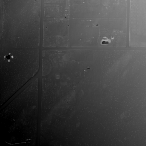
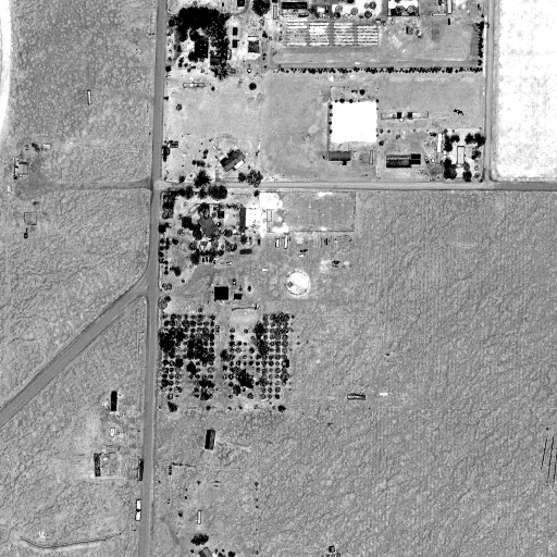
DEM // Ground level. Field boundaries and roads are visible, but flat-roofed and metal structures vanish due to laser scattering. |
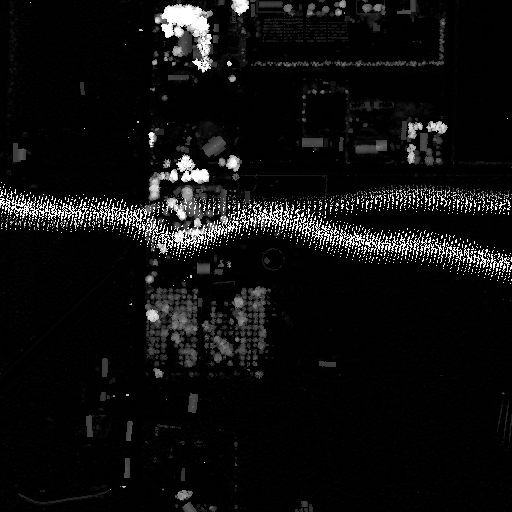
nDSM // Height above ground (DSM minus DEM). Structures and trees are bright against a black background, regardless of terrain elevation (please pardon the flight-line artifact). |
Laser Return Intensity // How strongly each laser bounced back. Metal and concrete roofs reflect brightly. |
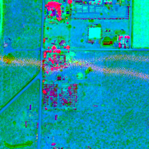
Combined: nDSM + Intensity + Planarity // Three channels mapped to RGB. Red = height above ground, Green = laser return intensity, Blue = surface smoothness. |
Each of these has their own benefits and drawbacks, however, with a combination of all of them, we can get a good view of what we're looking for.
// Using the data and training
Once the data is downloaded, laspy makes it easy to turn the data into numpy arrays for every point. Then, we can use rvt-py to make image tiles with the information we need in each channel, ready to be labeled and given to YOLO-v8 for training.
LabelImg made drawing bounding boxes with labels easy with a GUI frontend, however there was a problem with not much 'interesting' data being present in the 1000s of tiles I scanned through looking for things to label.
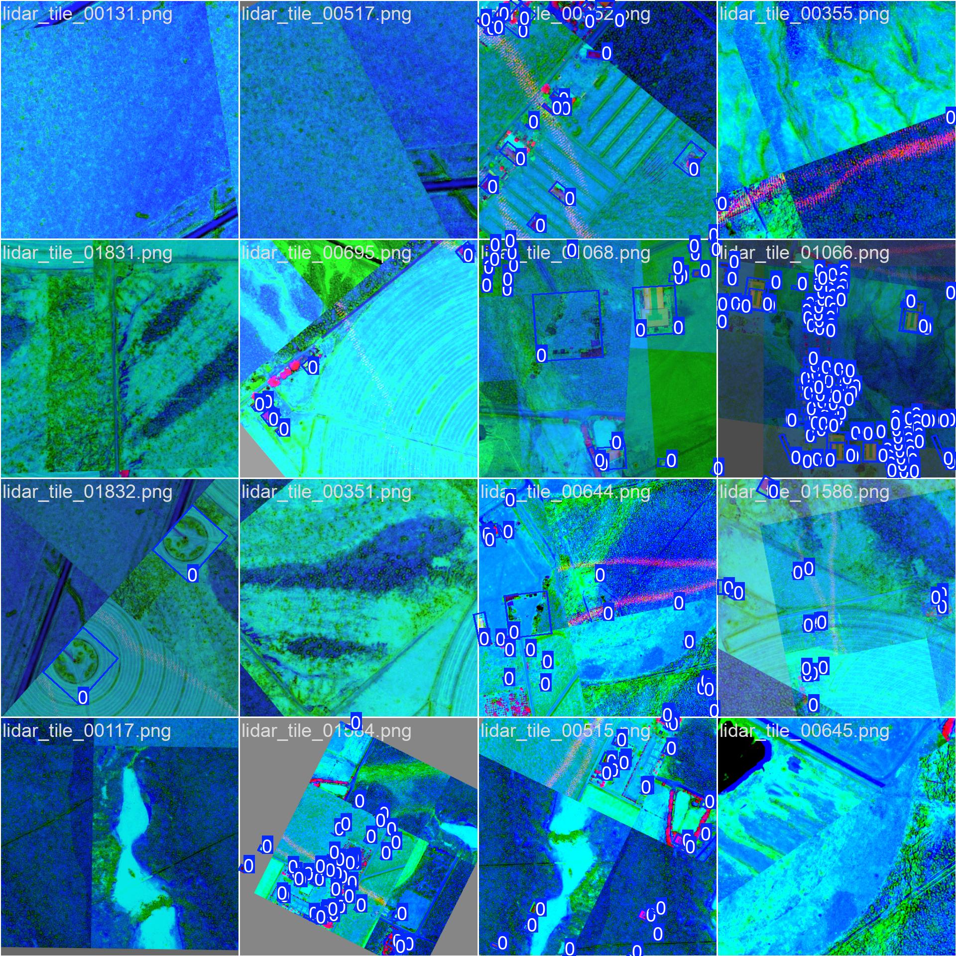
Labeled data to be used in the training pipeline. |
Once about 50 tiles were labeled (which ultimately wasn't enough), I used Ultralytics to locally train a YOLO-v8 model on what we had, which produced some cool graphs about the training progress.
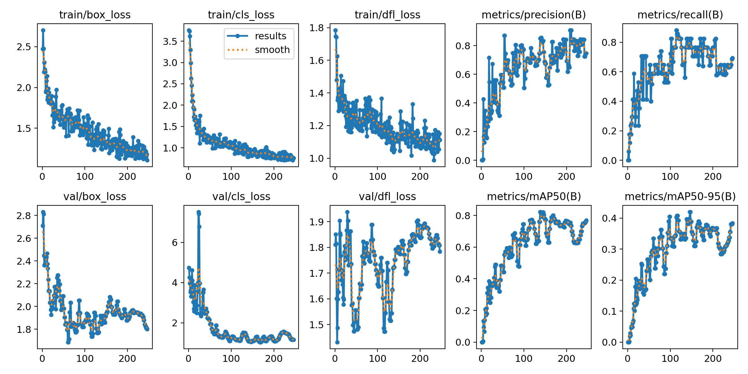
My first attempt at training a model locally -- lots of room for improvement here. |
Ultralytics will automatically keep track of the best performing model 'checkpoint' to avoid any problems with overfitting and return it as the result.
After training the model, we can see how it preforms on some test data.
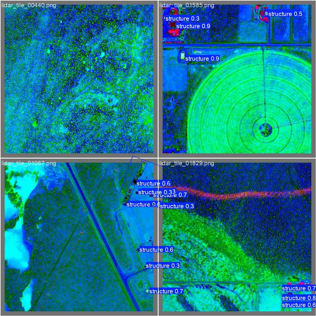
YOLO-v8 tuned labelling with confidence scores. |
// Conclusion
While my first foray into tuning a local model (and LiDAR), this project produced a small, ~58mb, OBB model that proved useful on data similar to the training data. However, the lack of labeled training data and consistency between LiDAR data being hard to manage for a solo exploratory project, made the effort relatively fruitless in terms of producing an image model to truly find everything. I would one day like to go back and look more into LiDAR visualization techniques and try to use AI-assisted labeling methods.